Neuron Models and Types

 Neuron Model and Network Architectures

Neuron Model:

A neuron with a single scalar input and no bias appears on the left below.

                           Fig.(1) Neuron Models

The scalar input p is transmitted through a connection that multiplies its strength by the scalar weight w, to form the product wp, again a scalar. Here the weighted input wp is the only argument of the transfer function f, which produces the scalar output a. The neuron on the right has a scalar bias, b. You may view the bias as simply being added to the product wp as shown by the summing junction or as shifting the function f to the left by an amount b. The bias is much like a weight, except that it has a constant input of 1.

The transfer function net input n, again a scalar, is the sum of the weighted input wp and the bias b. This sum is the argument of the transfer function f.

Here f is a transfer function, typically a step function or a sigmoid function, which takes the argument n and produces the output a. Examples of various transfer functions are given in the next section. Note that w and b are both adjustable scalar parameters of the neuron. The central idea of neural networks is that such parameters can be adjusted so that the network exhibits some desired or interesting behavior. Thus, we can train the network to do a particular job by adjusting the weight or bias parameters, or perhaps the network itself will adjust these parameters to achieve some desired end.

Activation Function Types

Many transfer functions can be used in neural networks Three of the most

commonly used functions are shown below.

 1- Linear:                         f (σ) = σ

 2- Hard- limit:                

                                 

3- Sigmoid:                   

                                 

 4- Hyperbolic:                

         

                            

  5- Perceptron:                

                                 

 The linear transfer function is shown below.

                           Fig.(2) Linear Transfer Function

The hard-limit transfer function shown below limits the output of the neuron

to either 0, if the net input argument n is less than 0; or 1, if n is greater than

or equal to 0.

                           Fig.(3) Hard-limit-transfer Function

The sigmoid transfer function shown below takes the input, which may have

any value between plus and minus infinity, and squashes the output into the

range 0 to 1.

Fig.(4) Log-Sigmoid Transfer Function

This transfer function is commonly used in back propagation networks, in part

because it is differentiable.

The symbol in the square to the right of each transfer function graph shown above represents the associated transfer function. These icons will replace the general f in the boxes of network diagrams to show the particular transfer function being used.

 Neuron With Vector Input

A neuron with a single R-element input vector is shown below. Here the individual element inputs.

p₁, p₂,... p_R. are multiplied by weights  [w1,1 , , w1,2 , , ... w1,R] .

and the weighted values are fed to the summing junction. Their sum is simply Wp, the dot product of the (single row) matrix W and the vector p.

                      Fig.(5) Neuron with Vector Input

The neuron has a bias b, which is summed with the weighted inputs to form

the net input n. This sum, n, is the argument of the transfer function f.

n=w1,1p1+w1,2p2+... + w1, RpR + b

This expression can, of course, be written in MATLAB code as:

n = W*p + b

The figure of a single neuron shown above contains a lot of detail. When we

consider networks with many neurons and perhaps layers of many neurons,

there is so much detail that the main thoughts tend to be lost. Thus, the authors have devised an abbreviated notation for an individual neuron. This

notation, which will be used later in circuits of multiple neurons, is illustrated

in the diagram shown below.

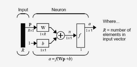
Fig.(6) Multiple Neuron

Here the input vector p is represented by the solid dark vertical bar at the left.

The dimensions of p are shown below the symbol p in the figure as Rx1. (Note that we will use a capital letter, such as R in the previous sentence, when referring to the size of a vector.) Thus, p is a vector of R input elements.

These Inputs post multiply the single row, R column matrix W. As before, a constant 1 enters the neuron as an input and is multiplied by a scalar bias b. The net input to the transfer function f is n, the sum of the bias b and the product Wp.

This sum is passed to the transfer function f to get the neuron’s output a, which in this case is a scalar. Note that if we had more than one neuron, the network output would be a vector.

A layer of a network is defined in the figure shown above. A layer includes the combination of the weights, the multiplication and summing operation (here realized as a vector product Wp), the bias b, and the transfer function f. The array of inputs, vector p, is not included in or called a layer.

As discussed previously, when a specific transfer function is to be used in a

figure, the symbol for that transfer function will replace the f shown above.

                          

SHARE

Ahmad Atiia

Hi. I’m Designer of Engineering Topics Blog. I’m Electrical Engineer And Blogger Specializing In Electrical Engineering Topics. I’m Creative.I’m Working Now As Maintenance Head Section In An Industrial Company.

• 
•