

The optimal power flow,
in general, is expressed as a nonlinear static optimization problem, the cost
function (Criterion) has various forms as follows:
1-Economic cost, where the cost function is C
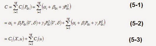
Where bus 1 is the
slack bus and buses 2, 3, ….., ng are ng generation buses. X = vector of state
variables (normally all bus angles except the slack bus angle and voltage
magnitudes of load buses). U = vector of control variables, (active generation
power except the slack generation and voltage of all generators). Here the
slack power generation is used as output variable.
2-Load Shedding Criterion, (the cost function is defied as "c")

where:

is the given load at bus i before load shedding.

is the control value
of the load at bus i.
NL is the number of load buses and Wi are assigned weights to different load buses, the criterion is used if the loads can not be met.
3-Pollution Criterion

Where Pi(PGi) shows the level of pollution
of generation i as a function of generation level.
The above functions eq's
(5-3)are minimized under set of equality and inequality constraints such as:
a)
The Equality Constraints
The equality constraints of
the problem can be expressed as the load flow equations plus slack generation
as:

The number of equations is
equal to the number of system state variables.
b)
The Inequality Constraints
1.Real generation constraints for
all generators

2.Voltage magnitude constraints for all
generators plus buses controlled by other control devices.

0.9 < Vi < 1.1 ( Normal
mode )
0.95 < Vi < 1.05 ( High quality mode )
0.98 < Vi < 1.08 ( Very High quality mode )
3. Reactive generation
constraints for all generation buses and other controlled buses.

4.
Security constraints on lines flows for all or specified lines.

The optimal power flow is
solved as constrained (all constraints are considered) or unconstrained (where
the inequality constraints are ignored) problem. The mathematical form of
unconstrained problem is:

The necessary optimality
conditions are given the Lagrange

The
suggested iterative scheme to solve the eq's (5-13)is:

A convergence is an curtained,
the optimum solution and optimal conditions are attained. Every iteration needs
a load flow solution, this may lead to a very computation time consuming. To
over come this problem and reduce the computation time, a matrix of second
partial derivation, Hussein matrix algorithm, is used.
Here, we define the
vector Z as:

As a result, the
Lagrange is a function of Z, i.e.,

The necessary
optimality conditions become simply

Defining the Hussein
matrix H(Z) of partial derivations as:

Then the Newton-Raphson
iterative procedure becomes

By choosing a good initial
vector Z, this approach should converge very quickly. For a large system, the
matrix H is sparse. Hence, sparse matrix methods are applicable. Since Z is
>> 2.5 times larger than the vector X of state variables, solution times
for this OPF approach should be two to three times greater than the
corresponding load flow problem.
OPF Algorithm's Flow Chart :

Hi. I’m Designer of Engineering Topics Blog. I’m Electrical Engineer And Blogger Specializing In Electrical Engineering Topics. I’m Creative.I’m Working Now As Maintenance Head Section In An Industrial Company.
0 comments:
Post a Comment