

In this section, a simple derivation is made for
an approximately loss function. First, a expression of line losses in terms of
high voltages and phase angles is made. Let Pij , denote real power flow from
bus i to bus j. From the load flow equations, one can write:

By adding these two equations, one obtains the
loss for line (i-j):
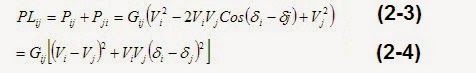
If all voltages are at nominal values, (e.g.
base voltages) then:
 as a result
Let M denote the line-bus incidence matrix with
order NL×N if the slack bus is included
where NL and N are number of system lines and buses respectively with [S] = [S1
S2 … Sn]t. Also, let Y denote the vector of angular differences across all lines with order NL×1, then one can write:

Let G be a diagonal matrix of line conductance's
with order NL × NL , i.e.:

It is possible to use equations from (2-1) to
(2-7) to show that line losses are given by:

The vector d can be approximated by the
DC load flow approach, with:


for i=1….N and the
vector d has elements di for i=1...... N and the matrix A has dimensions N×N.
As a result, using eq. (2-6), eq. (2-8) and eq.
(2-9) line losses become:

The vector PG has dimensions n×1,
and the vector PD has dimensions n×1
which have the generation and demands at all system buses.
Thus, in an approximate manner, PL is a
quadratic function of PG. The expression for PL is known as a loss formula.
There are a variety of other loss formula depending on the degree of
approximation employed. It is clear that system losses depends strongly on the
matrix B (known as the B-Coefficient matrix), this matrix is strongly dependent
on the system topology (both M and A dependent), and the network admittance's (G
is dependent on line conductance and A on susceptances).
Eq. (2-13) can be rewritten for n power plants
as:

Where: Pi and Pk are the power outputs at buses
i and k respectively. [P]t vector of [P1, P2, ……, Pn]t with order n where the
element i for example is equal PGi-PDi and the B coefficient matrix is given
by:

The elements of matrix B are function of the
line resistance's and reactance and the system operating point.
On the other side, there are other forms of loss
formula as below the complex power at bus i is:
Then the complex power loss of the system in
terms of bus admittance or bus impedance is:
For bus impedance form with:

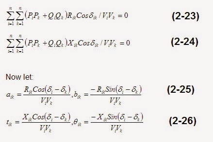
Where Rik, Xik are resistance and reactance of line connected between bus i and bus k
respectively, di , Vi are bus voltage angle and
magnitude at bus i. Equation (2-20) reduces to give the active PL, and
reactive, QL, system loss as:

The complex form of power loss given by
eq.(2-20) can be given in matrix form as:

Where P and Q are bus power vectors and a, t, q and d are n×n matrices.
The generation units penalty factors are:

Hi. I’m Designer of Engineering Topics Blog. I’m Electrical Engineer And Blogger Specializing In Electrical Engineering Topics. I’m Creative.I’m Working Now As Maintenance Head Section In An Industrial Company.
0 comments:
Post a Comment